Following my second Tableau project, I am continuing my journey with Data Career Jumpstart to analyze real data from the manufacturing/industry sector using Python.
Key Findings and Recommendations for Plant Management
- Airflow measurements at Columns 4 and 5 show minimal variability (IQR near zero), indicating either strict control or a potential sensor malfunction. It is recommended to verify the sensors’ functionality and confirm whether these columns are operating as intended.
- The level variability for Column 3 was the highest. It is recommended to look into whether this might a sensor problem, or if Column 3 is purposely designed to handle variations in the flotation process.
- Performance evaluations should not rely only on final concentrate numbers. Instead, use data from mid-August as an operational benchmark to demonstrate that the plant can handle worst-case scenarios.
- Consider sourcing feed ore as a strategic plan for quality. Data from the end of May to the beginning of June indicates that premium ore produces a cleaner product with minimal processing.
- The plant produced consistent product quality between day and night shifts.
Flotation is a technique used to separate valuable minerals from gangue. It takes advantage of differences in how these materials behave on the surface. This method helps extract metals from low-grade and complex ores, making it important for various industries, including electronics and renewable energy.[link]
The dataset was a real industrial dataset and was accessible on Kaggle [link]. Each row in the dataset represents the plant’s operational state at a specific time. The data has 737,453 rows, recorded from March 10, 2017, to September 9, 2017.
The Python code for this project can be found here >>
The Goal
This analysis seeks to understand why quality varies and which operational steps are the most significant. By examining equipment performance, the relationship between feed and product, time-related patterns, and performance at the shift level, the goal is to uncover actionable insights. These insights can help plant managers improve consistency and ensure effective quality control.
The Approach
The analysis is organized around five key questions that enhance understanding of the process.
- Comparing Flotation Columns: Are all seven columns behaving consistently or are some operating differently than others?
- Feed vs. Final Product Quality: Does the quality of raw ore directly determine final product quality?
- Tracking Performance Patterns Over Time: How consistent is the rolling weekly process and are there times of significantly better or worse performance?
- Measuring Process Efficiency: Beyond final quality numbers, how efficiently does the plant enrich iron and remove silica relative to what it is fed?
- Performance by Time of Day: Do day and night shifts produce different results?
In the end, the objective is not only to understand the data, but also to translate patterns into actionable recommendations for plant management to investigate or implement.
Initial Findings and Decision
By examining the first and last few rows of the dataset, I found that some values were duplicated across several columns, including the % Iron Feed, % Silica Feed, % Iron Concentrate, and % Silica Concentrate columns. This observation aligns with the data source’s description, which indicates that some columns were sampled every 20 seconds, while others were sampled hourly.
To confirm the number of duplicates for all columns, I ran the nunique function and get the results below.
date                              4097
% Iron Feed                        278
% Silica Feed                      293
Starch Flow                     409317
Amina Flow                      319416
Ore Pulp Flow                   180189
Ore Pulp pH                     131143
Ore Pulp Density                105805
Flotation Column 01 Air Flow     43675
Flotation Column 02 Air Flow     80442
Flotation Column 03 Air Flow     40630
Flotation Column 04 Air Flow    196006
Flotation Column 05 Air Flow    194711
Flotation Column 06 Air Flow     90548
Flotation Column 07 Air Flow     86819
Flotation Column 01 Level       299573
Flotation Column 02 Level       331189
Flotation Column 03 Level       322315
Flotation Column 04 Level       309264
Flotation Column 05 Level       276051
Flotation Column 06 Level       301502
Flotation Column 07 Level       295667
% Iron Concentrate               38696
% Silica Concentrate             55569
dtype: int64
Decision
Since duplicate timestamps occurred at hourly intervals rather than every 20 seconds, all columns were aggregated to hourly intervals by averaging their values for each hour.
Analysis
1. Comparing Flotation Columns

* Outliers are not displayed in the boxplots.
At first, I intended to analyze the data based on median values. However, after plotting the boxplots for each column, it shows that the medians alone were not informative enough. Air flow medians were nearly identical across all columns, and level medians showed only two broad groupings (columns 1–3 vs. columns 4–7). Hence, I shifted focus to IQR (interquartile range) as a measure of variability, since the spread between Q1 and Q3 showed more differences across both air flow and level columns.

The two charts show that air flow and levels in the columns do not change in the same way.
Air Flow
There are 3 groups of pattern here:
- Columns 1–3 had high, nearly identical variability, with a middle 50% range of about 50 units, indicating similar operating conditions.
- Columns 4 and 5 show almost no variability (IQR close to 0), suggesting that airflow was either consistently maintained or that the sensors were not capturing changes. We need to confirm this with the plant manager.
- Columns 6 and 7 had moderate variability, around 30 and 17 units, respectively.
Levels
Generally, the variability in levels decreased as the process moved from one column to the next. However, the pattern changed in Column 3: instead of showing lower variability than Column 2, it shows the highest variability, nearly reaching 200 units. This finding needs to be reported to the plant manager to determine whether Column 3 is functioning properly or if it is intentionally designed to operate more variably.
2. Feed vs. Final Product Quality
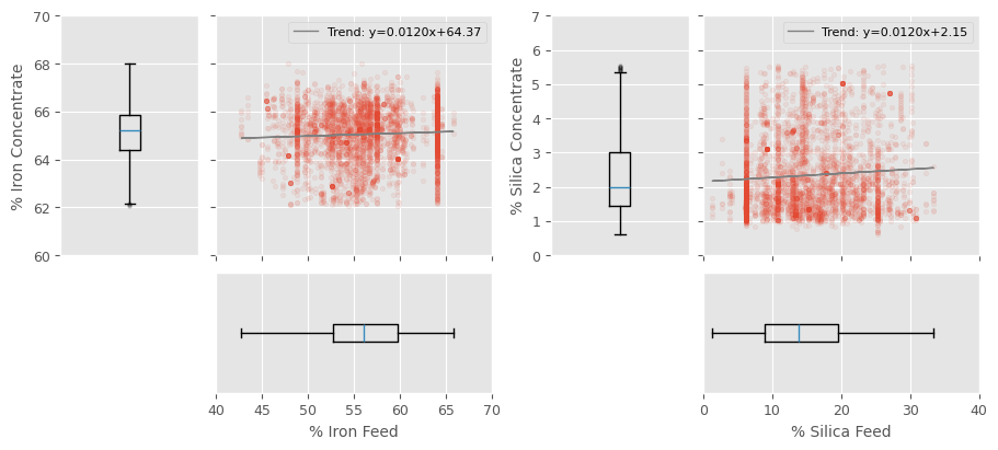
* The scatter plots show distinct clusters in the vertical banding patterns observed along the axes for % Iron Feed and % Silica Feed axes, which are likely due to hourly sampling.
Boxplot
The boxplots illustrate the transformation that takes place during the flotation process:
- The % Iron Feed ranged from 43% to 66%, with a median of 56%. In contrast, the % Iron Concentrate was tightly controlled, ranging from 62% to 68%, and had a median of 65%. This process effectively transforms a highly variable feed into consistently high-grade product, reducing the 23-percentage-point difference in the feed to just 6 points in the concentrate.
- The % Silica Feed varied significantly, ranging from 1% to 33%. Despite this wide variation, the output consistently remained below 6%, with a median of only 2%. The flotation circuit effectively eliminated most of the silica contamination, minimizing the 32-point range in the feed to just a 6-point range in the concentrate.
Scatter Plot
The boxplots illustrate the overall ranges of the data, while the scatter plots show whether individual data points follow a predictable pattern. Both iron and silica exhibit trend line slopes of 0.012, which means that for every 10 percentage point increase in feed, the concentrate increases by only 0.12%.
This weak connection supports what we see in the boxplots: the flotation process helps maintain consistent results, even when the raw materials used vary. Whether the iron content in the feed is low (43%) or high (66%), the final product contains about 65% iron. Similarly, regardless of whether the silica content in the feed is lower (1%) or higher (33%), the final product consistently contains around 2% silica.
3. Tracking Performance Patterns Over Time
To capture the ‘normal’ pattern in the Floatation plant, I applied a moving average [link]. This statistic gives insight into the data to identify trends and anomalies over time.
Iron Concentrate Trend (7-Day Moving Average)
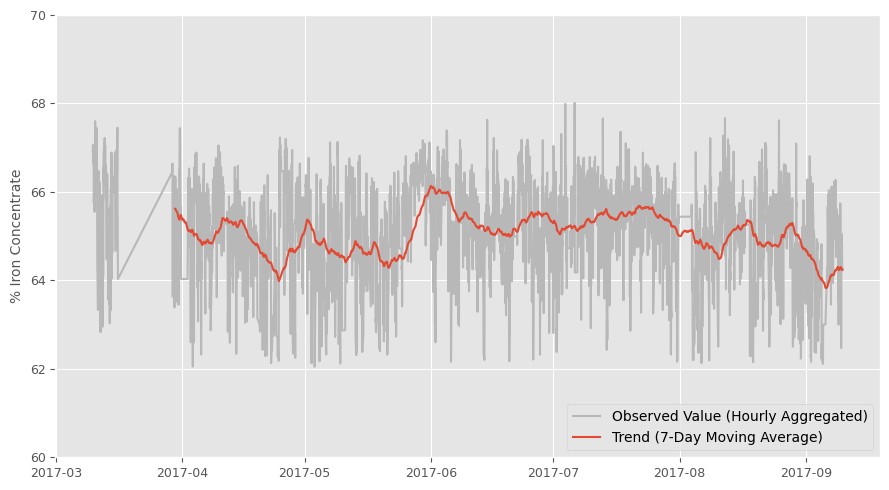
From the hourly data (represented by the gray line), I observed spikes reaching 68% and dips as low as 63%. However, the weekly moving average trend shows that the percentage of iron concentrate is generally between 64% and 66%, indicating a relatively flat overall trend. This suggests that while the process may be inconsistent at the hourly level, it operates within a general range over time.
The most notable jump is a climb in the trend line around the beginning of June 2017. This is worth investigating. It may be due to changes in feed quality or to different processing conditions during that period.
Silica Concentrate Trend (7-Day Moving Average)

The Silica Concentrate chart shows more noticeable oscillations, with hourly readings ranging from nearly 0% to 5.5% throughout the period. This variability makes Silica a more challenging variable to manage since higher silica levels are generally undesirable in iron ore output, as they indicate impurity.
The 7-day moving average for Silica starts relatively high, around 2.5% to 3.5%, from mid-April through mid-May. It then drops sharply to its lowest point, approximately 1.3% to 1.5%, at the beginning of June before gradually rising back to 2.5% to 3% by the end of August. This behavior may be linked to variations in feed material, such as seasonal ore quality, or a process adjustment made in June that was later reversed.
The dip in June stands out as the most favorable period, where both the trend and hourly readings were at their lowest. Since the main objective of a floatation plant is to minimize silica content, understanding what changed at the beginning of June could be beneficial for the plant manager.
4. Measuring Process Efficiency
Section 2‘s scatter plot analysis revealed an important finding: both iron and silica showed extremely weak correlations between the feed and final concentrate. With slopes of 0.012 for both, it suggests that the flotation process largely standardizes the output regardless of input quality.
However, the scatter plots couldn’t show us when the process is really putting in effort compared to when it’s just getting by. If the quality of the final product stays about the same, no matter whether we have good or bad raw materials, how can we tell if the process is actually working well?
This is where we look at how well things are working. Instead of focusing only on the final products, we measure the changes that occur along the way. This helps us understand the hard work that goes into the flotation process, even when it isn’t always visible.
Feed Quality Over Time
To better understand the process, first, we need to examine the variations in feed composition over time.

The feed composition charts reveal variation in ore quality:
- % Iron Feed ranged from 49% to 65%:
- The period from the end of May to the beginning of June 2017 had the highest-grade ore (~65%)
- The middle of August saw depleted ore (~49%)
- % Silica Feed varied from 6% to 25%:
- The period from the end of May to the beginning of June 2017 featured the cleanest ore (6% silica)
- The middle of August 2017 had the dirtiest ore (25% silica)
These feeding patterns give additional context for understanding product quality and process efficiency.
Connecting Feed, Efficiency, and Final Product Quality
To measure process efficiency, I calculated 4 metrics: iron efficiency, silica reduction, % iron recovery [link], and silica removal rate [link], defined by the formulas below.

* Hourly data were aggregated weekly: each bar represents the average of the aggregated hourly data. The median line was determined from the initial hourly aggregation, rather than from the weekly aggregation used for the bar chart.
Note on aggregation: The efficiency bar charts present weekly averages (using fixed calendar weeks), whereas the earlier time series used 7-day moving averages (with continuous windows). Both formats convey the same information but from different temporal perspectives.
Analyzing all three data sources (feed composition, efficiency metrics, and product concentrate) tells the complete story.
Period A: From the end of May to the beginning of June 2017
In this period, the 7-day moving average trend lines indicated that % Iron Concentrate peaked at 66%, while % Silica Concentrate dropped to between 1.3% and 1.5%, marking the lowest sustained level. However, efficiency bar charts raised concerns: Iron Efficiency was only 1%-2%, compared to a median of 8.9%, and Silica Reduction ranged from 3% to 5%, with a median of 11.4%.
The feed composition helps explain these figures: it consisted of 64-65% iron (the highest level) and 6% silica (the lowest level).
This analysis suggests that period A’s clean concentrate was a result of using premium ore rather than true process excellence. With the feed already containing 64% iron and only 6% silica, minimal effort was required to achieve a concentrate with 65-66% iron and 1.5% silica.
Period B: The middle of August 2017
During this period, the 7-day moving average trend lines for the % Iron Concentrate remained steady at 65%, while % Silica Concentrate increased to 2%-3%. However, the efficiency bar charts indicated that % Iron Recovery reached 133%, and Silica Removal Rate achieved 92%, the highest in the dataset.
The feed composition provides insight into these results: it consisted of 49-55% iron (the lowest level) and 25% silica (the highest level, four times that of period A).
In summary, period B had the lowest feed quality recorded, yet operational performance remained strong through exceptional efforts. It showcases operational excellence under challenging conditions.
When managing a flotation plant, it’s important not to evaluate its performance only based on the final product concentration. Also, consider sourcing feed ore as a strategic aspect. While this may not significantly improve the final product quality (according to a scatter-plot analysis), it can help reduce the processing burden to achieve that quality. Premium ore, such as period A’s, enables the plant to operate more smoothly, while challenging ore, such as period B’s, forces the process to operate at maximum capacity.
5. Performance by Time of Day

The gap charts for both % Iron Concentrate and % Silica Concentrate indicate that the difference typically ranges from 1% to +1%, with most values centered around zero. This suggests that the plant operates consistently both during the day and at night. Therefore, it appears that the factors influencing quality are more likely related to other aspects of the process than to operational differences between shifts.