Zoom Through the New Normal Taxi Trips
13 March 2023
Data Cleaning and Exploratory Data Analysis (EDA) on The Last One Year of Chicago Taxi Trips Dataset
As the pandemic slowly recedes, people are starting to travel more. They are revisiting their families and holiday destinations, and with businesses reopening, they are resuming their weekday commutes. Due to those reasons, it will be interesting to see the current mobility patterns: travel patterns after the pandemic.
This project focuses on observing taxi rides, a type of transportation anyone can access. But, unlike public transportation, taxis do not have specific schedules or routes, so the data collected can provide insight into trips taken throughout various neighborhoods at all hours of the day and night.
Though it will be interesting to look at the effects of the pandemic on the taxi industry, this project is limited to the last one-year’s taxi trips only. The data analysis will not include taxi trips from before or during the pandemic when stay-at-home orders were in effect.
This project involves two processes to determine the current mobility pattern: data cleaning to enhance data quality and exploratory data analysis (EDA) to describe trip characteristics.
Dataset
This project will study the taxi trips in the Chicago Taxi Trips Dataset, one of the datasets available on the Chicago Data Portal. While working on this project, the dataset contains taxi trip data from 2013 to 2023.
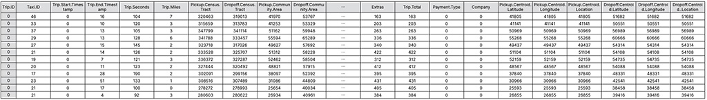
We can potentially study when the trip happened, the duration and distance, the pickup and dropoff location, the amount paid, the payment method, and the taxi company from each record of this dataset. Below is the description for all variables arranged into eight broad groups.
- ID
Two IDs in the dataset, Trip.ID and Taxi.ID, are the unique identifiers for the trip and the taxi. - timestamp
Trip.Start.TimeStamp and Trip.End.Timestamp show when the trip started and ended. The time is rounded to the nearest 15-minute interval to avoid passenger reidentification. - duration of the trip
Trip.Seconds shows trip duration in seconds. - distance of the trip
Trip.Miles marks travel distance in miles. - location
Pickup.Census.Tract, Pickup.Community.Area, Pickup.Centroid.Latitude, Pickup.Centroid.Longitude, and Pickup.Centroid.Location (point of both latitude and longitude) depict the pickup location. At the same time, the Dropoff.Census.Tract, Dropoff.Community.Area, Dropoff.Centroid.Latitude, Dropoff.Centroid.Longitude, and Dropoff.Centroid..Location (point of both latitude and longitude) represent the dropoff location.
These locations are imprecise to protect the passengers’ privacy. Moreover, the record was blank for locations outside Chicago. - payment amount
The trip costs are in Fare, Tips, Tolls, Extras, and Trip.Total columns. - payment type
Payment.Type variable tells the payment method. - taxi company
The Company column has the taxi company information.
As a public dataset, Chicago Taxi Trips Dataset is available for anyone to access and use.
Prepare
Select the relevant data
This project aims to clean and perform exploratory data analysis (EDA) for the last one-year data of the Chicago Taxi Trips Dataset. Since I conducted this project in March, this project covers the period from March 2022 to February 2023.
After downloading 12 months of records from the Taxi Trip page in the Chicago Data Portal, I managed to get more than 6 million rows of raw data.
Identify problems in the dataset
To accurately convey the insight from the data, having a clean one is crucial. Not only ensure the reliability of the prospective statistical analysis, early identified and resolved issues will simplify it.
The methods to pinpoint the issues from the data are listed below.
- Confirm the dataset completeness
- Look for duplicate
- Determine irrelevant column
- Locate missing value
- Spot any outliers
- Review datatypes
Confirm the dataset completeness
To reasonably illustrate the trip patterns throughout the year (12 months), I must ensure the data covers virtually all the days in each month. For this project, I defined a month as complete if it has: (1) the first day of the month, (2) the last day of the month, and (3) 90% of the total days (26 out of 28 days, 27 out of 30 days, or 28 out of 31 days).
# Sort dataset based on the time the trips were started,
# then and print (1) the the first and last row, and (2) number of unique days in each month
for (i in 1:12) {
  df <- eval(parse(text = paste0("raw_df_", i) )) %>% arrange(Trip.Start.Timestamp)
  n_days <- n_distinct(substr(df$Trip.Start.Timestamp, 1, 10)) - 1
  print(paste0("first: ", min(df[1, 3]), " - last: ", max(df[nrow(df), 3]), " - n_days:  ",  n_days))
  rm(df)
}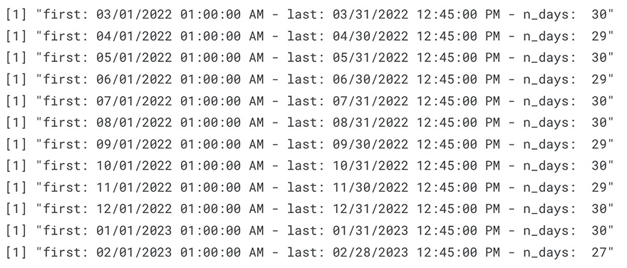
The image above shows that, by my definition, the datasets are complete.
Look for duplicate
Chicago Taxi Trips Dataset owns a unique primary key, Trip.ID, that avoids data duplication. Still, I performed this duplicate finding process to confirm that supposition.
for (j in 1:12) {
    df <- eval(parse(text = paste0("raw_df_", j)))
    if (dim(df %>% distinct())[1] == dim(df)[1]) {
        print(paste0("month ", j, ": no duplicate"))
    } else {
        print(paste0("month ", j, ": has duplicate"))
    }
    rm(df)
}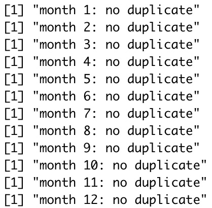
From the result above, we can conclude that no duplicated row exists in the dataset.
Determine irrelevant column
Unique identifications will be unnecessary for later analysis. Thus, I will remove Trip.ID and Taxi.ID. Furthermore, I will only keep the Pickup.Centroid.Location and Dropoff. Centroid..Location among all location variables since they already have latitude and longitude information for the census tract or community area.
Locate missing value
table <- data.frame(raw_df_1)
missing <- table %>% sapply(function(x) sum(is.na(x) | x == ""))
rm(table)

for (i in 2:12) {
    table <- eval(parse(text = paste0("raw_df_", i)))
    missing <- missing %>% rbind(table %>% sapply(function(x) sum(is.na(x) | x == "" )))
    rm(table)
}
Two forms of missing values, the no value available (NA) and the blank space (“”), were in this raw dataset.
Spot any outliers
Outliers are extreme values in data that were far from the other values. These values can skew the data and affect the accuracy of statistical analyses.
We can spot the outliers using a box plot. Unlike previous identification, I combined datasets from all 12 months to spot outliers.
## List of numeric columns
num_cols = list("Trip.Seconds", "Trip.Miles", "Fare", "Tips", "Tolls", "Extras", "Trip.Total")

## Box Plot with outliers marked in red
myplot <- function(col){
    raw_df %>% na.omit() %>%
        ggplot(aes(y= eval(parse(text = col))))  +
        geom_boxplot(outlier.colour = "red", outlier.shape = 1)+
        labs (x = col, y = "") +
        theme(axis.text.x = element_blank())
}

## Plot all numeric columns
plot_list <- lapply(num_cols, myplot)

ggarrange(plotlist = plot_list,
          nrow = 5, ncol = ceiling(length(plot_list)/5))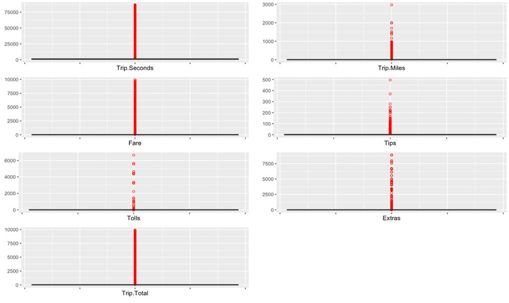
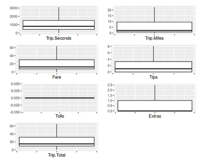
Boxplot shows that all numeric columns in raw dataset contain outliers (the red circles).
Review datatype
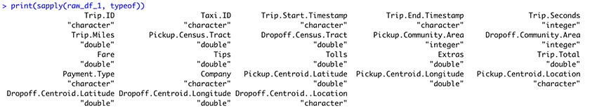
From the figure above, we can see that some columns have wrong datatypes.
- The Trip.Start.Timestamp and Trip.End.Timestamp should have a date-time type instead of a character.
- The Pickup.Centroid.Location and Dropoff.Centroid..Location must be converted to points; hence we can position them on a map.
Data Cleaning
After identifying all problems in the data, the next step is to fix them.
Remove irrelevant columns
This procedure removed ten of all the variables in the data: Trip.ID, Taxi.ID, Pickup.Census.Tract, Dropoff.Census.Tract, Pickup.Community.Area, Dropoff.Community.Area, Pickup.Centroid.Latitude, Pickup.Centroid.Longitude, Dropoff.Centroid.Latitude, and Dropoff.Centroid.Longitude.
df <- df %>%
    subset(select = -c(Trip.ID, Taxi.ID, Pickup.Census.Tract, Dropoff.Census.Tract, Pickup.Community.Area, Dropoff.Community.Area, Pickup.Centroid.Latitude, Pickup.Centroid.Longitude, Dropoff.Centroid.Latitude, Dropoff.Centroid.Longitude))
Handle missing values
I address the missing values problem by deleting the rows containing them. This procedure is doable since the taxi trip datasets have many rows.
# Drop missing values
df[df == ""] <- NA
df[df == ""] <- NA
df <- df %>% drop_na()
This process removed 896,438 rows (13.64%) of data.
Handle the outliers
Capping their value is one way to handle outliers: replacing the outliers’ values with the upper bound and lower bound.
This technique utilizes the Interquartile Range (IQR) of the data. The IQR is a measure of the spread of the data. It is the difference between the data’s third quartile (Q3) and the first quartile (Q1). Any data point that falls below the lower bound (Q1 – 1.5 * IQR) or above the upper bound (Q3 + 1.5 * IQR) is an outlier, and the lower or upper bound can replace their value, respectively.
for (col in num_cols) {
    Q <- quantile(df[[col]], probs = c(.25, .75))
    iqr <- IQR(df[[col]])
    upper_bound <-  Q[2] + 1.5*iqr
    lower_bound <- Q[1] - 1.5*iqr

    df[[col]] <- ifelse(df[[col]] > upper_bound, upper_bound, df[[col]])
    df[[col]] <- ifelse(df[[col]] < lower_bound, lower_bound, df[[col]])
}
No red circles on the boxplots indicate no outliers —their values have been substituted with lower or upper bound values.
Change columns datatypes
timestamp
The datatype of Trip.Start.Timestamp and Trip.End.Timestamp were converted from a string into a date-time datatype using the lubridate library.
df$Trip.Start.Timestamp <- df$Trip.Start.Timestamp %>% parse_date_time("%m/%d/%y %I:%M:%S %p", tz = "America/Chicago")
df$Trip.End.Timestamp <- df$Trip.End.Timestamp %>% parse_date_time("%m/%d/%y %I:%M:%S %p", tz = "America/Chicago")
The new datatypes for Trip.End.Timestamp and Trip.End.Timestamp are POSIXct.
location
The string on Pickup.Centroid.Location and Dropoff.Centroid..Location were converted to latitude-longitude points by utilizing the simple feature library.
df <- df %>% st_as_sf(wkt = "Pickup.Centroid.Location")
df <- df %>% data.frame() %>% st_as_sf(wkt = "Dropoff.Centroid..Location")
The new datatypes for ‘Pickup.Centroid.Location’ and ‘Dropoff.Centroid..Location’ are sfc_POINT.
Exploratory data analysis (EDA)
Summary statistics
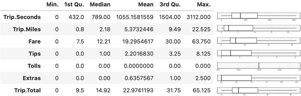
The median, mean, and boxplot show that all the variables have right skew distribution except Tolls that only have value of zero.
Trip.Seconds (TRAVEL TIME)
The average taxi trip took almost 18 minutes, and nearly half were less than 13 minutes.
Trip.Miles (TRAVEL DISTANCE)
The average travel distance was around 5.3 miles, and half were less than 21/4 miles. Less than 1/4 of trips were farther than 9.5 miles.
Fare
On average, one trip by taxi costs $19.3. Half of the trips cost between $7.5 to $30.
Tips
On average, passengers gave $2.2 tips, about $1 more than the median.
Tolls
The passengers paid no toll.
Extras
On seventy-five percent of the trips, passengers paid $1 or fewer extra payments.
Trip.Total (TOTAL Payment)
The median of total payment was almost $15, nearly $3 more than the median fare. About a quarter of the trips, passengers paid more than $32.
Distribution of values in a single variable
Date and time
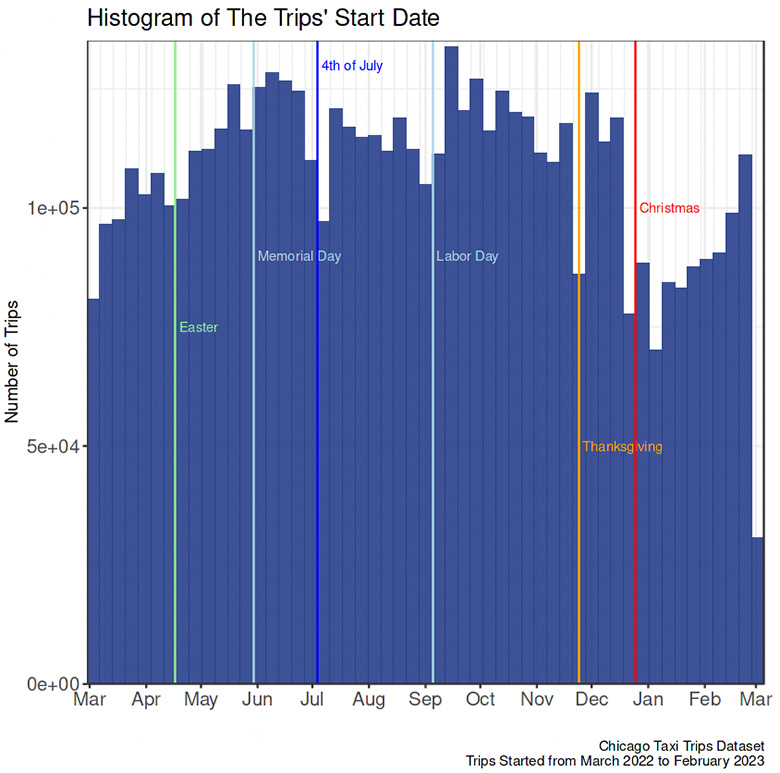
- Each bar on the graph above covers one week, and the height indicates the number of trips in each time range. The histogram starts during the week of March 1, 2022, and ends during the week of February 28, 2023. The week begins on Sunday and ends on Saturday.
- The first week and the last off were incomplete, hence the lack of trips compared to the closest week.
- Interestingly, compared to the week before and after, there were fewer taxi trips during the holidays: Easter, Memorial Day, 4t of July, Labor Day, Thanksgiving, and Christmas. It may be because fewer people rode taxis during holidays or fewer drivers worked during holidays.
- There was an unknown reason for the decreasing number of trips in the second week of January 2023.
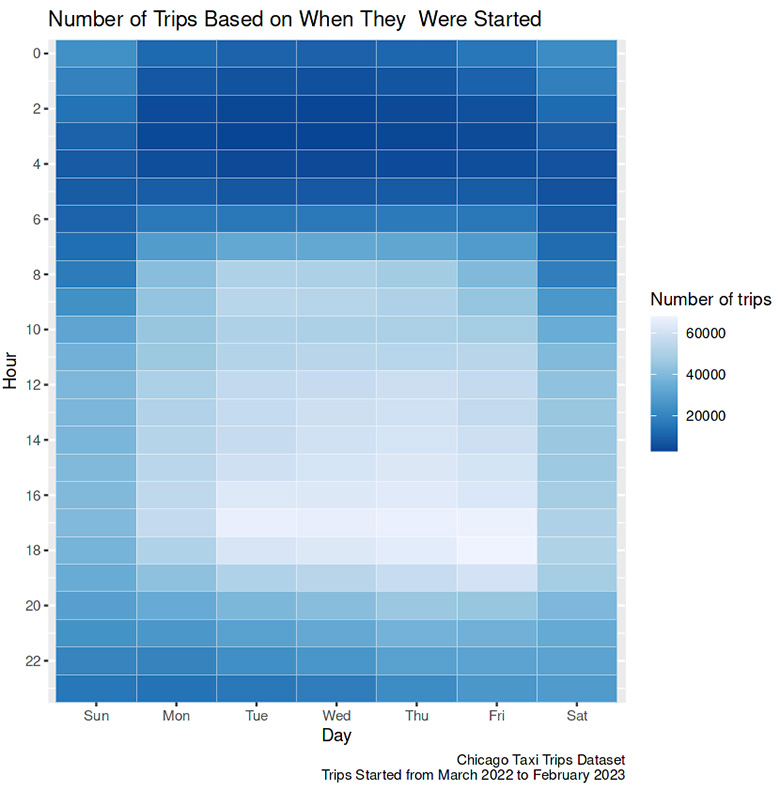
- Compared to the day, more people rode a taxi at night.
- On the weekend, night trips peaked later, closer to morning.
Travel time
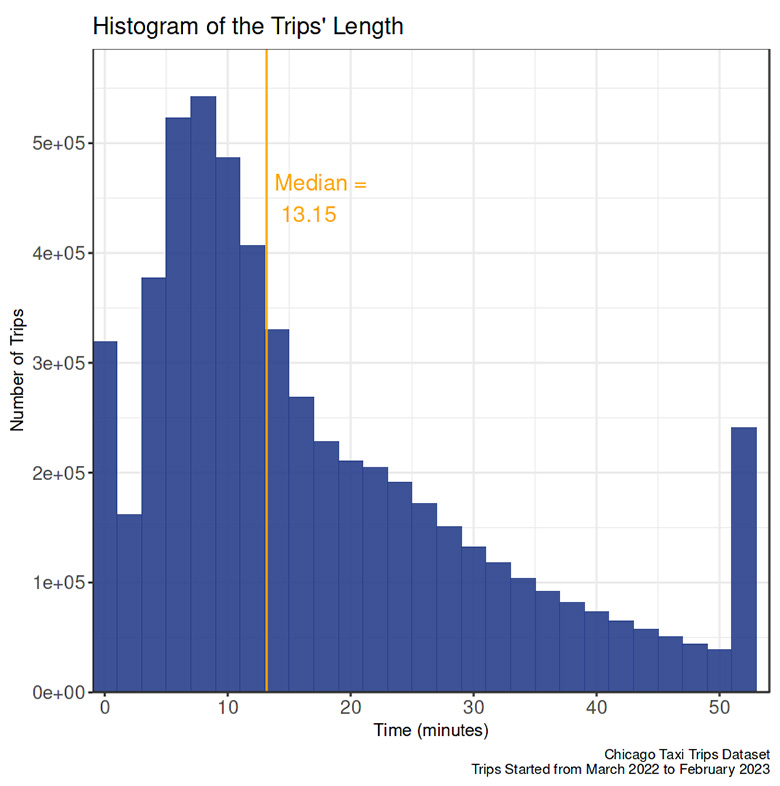
- The histogram is right-skewed.
- The most considerable frequency of trips is in the 7-9 minutes range.
- More than half of the trip was less than 15 minutes.
- The data cleaning process substituted outliers’ values with the upper bound. The increased number of trips at the end of the histogram means that the histogram will have quite a long tail without the substitution.
Travel distance
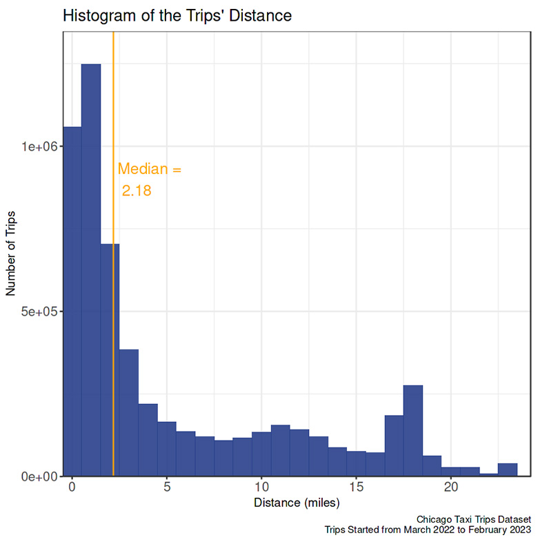
- The taxis were unlikely to travel more than 20 miles.
- The highest number of taxi trips is in the 0.5 to 1.5 miles range.
Fare
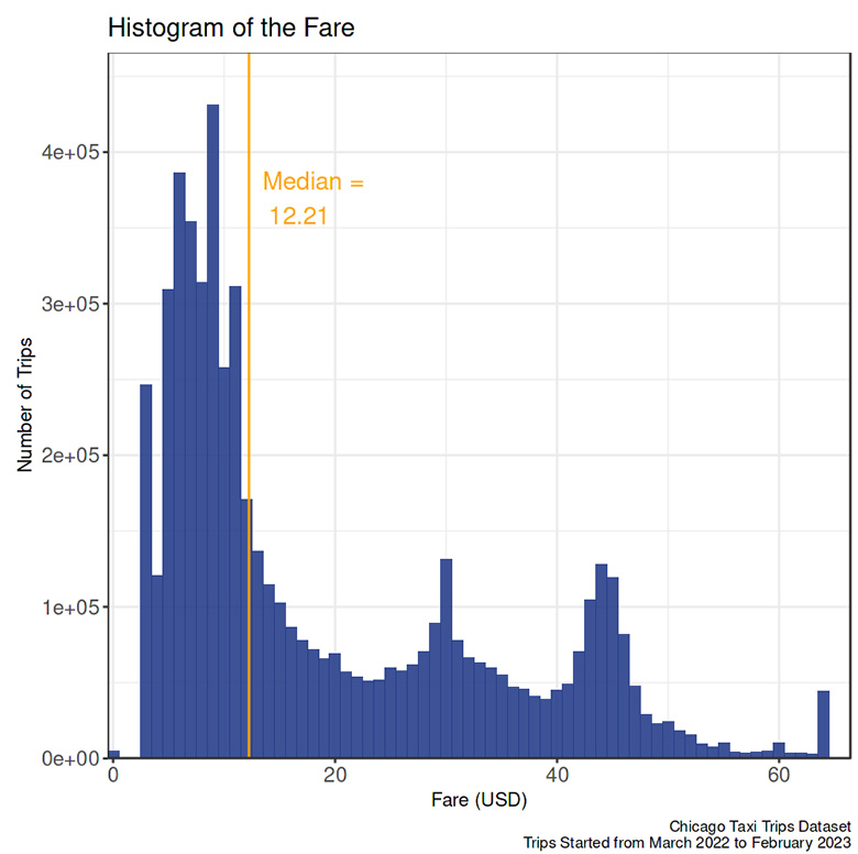
- In this graph, the increase in the histogram’s end due to substituting outliers’ values with the upper bound was also observable.
- Several peaks, known as multimodal, appear in the histogram. The highest number of trips is in the $8.5 to $9.5 range, with a longer tail to the right than the left. The smaller peaks are $29.5 to $30.5 and $43.5 to $44.5. This multimodal phenomenon needs further investigation beyond exploratory data analysis.
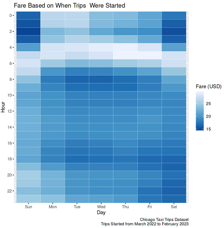
- Fare also varied based on the time of the day. The trips were cheapest in the early morning and most expensive on weekends late at night. An hourly taxi distance and speed comparison is needed if we want to know why these fare variations exist.
Tips
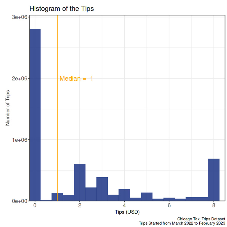
- On all trips, the passenger likely gave no tips to the taxi driver.
Extras
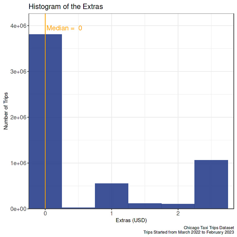
- In most trips, taxi riders paid no extra charge.
Total Payment
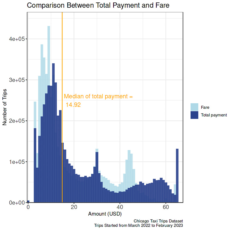
- Similar to the fare distribution, the total payment distribution has three peaks. The comparison makes it more apparent that three groups of unknown categories differentiate the fare. In the first group, the total payment (peak in the $10.5 to $11.5 range) is noticeably higher than the fare (peak in the $8.5 to $9.5 range); in the second group, the total payment (peak in $29.5 to $30.5 range) is almost equal to the fare (peak in $29.5 to $30.5 range), while in the last group, the total payment is remarkably higher than the fare (peak in $43.5 to $44.5 range).
Payment methods

- The most popular payment method was credit cards, while the least was prepaid.
Company
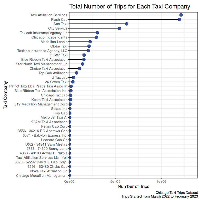
- The two most popular taxi companies were Taxi Affiliation Services and Flash Cab.
Pickup and dropoff locations
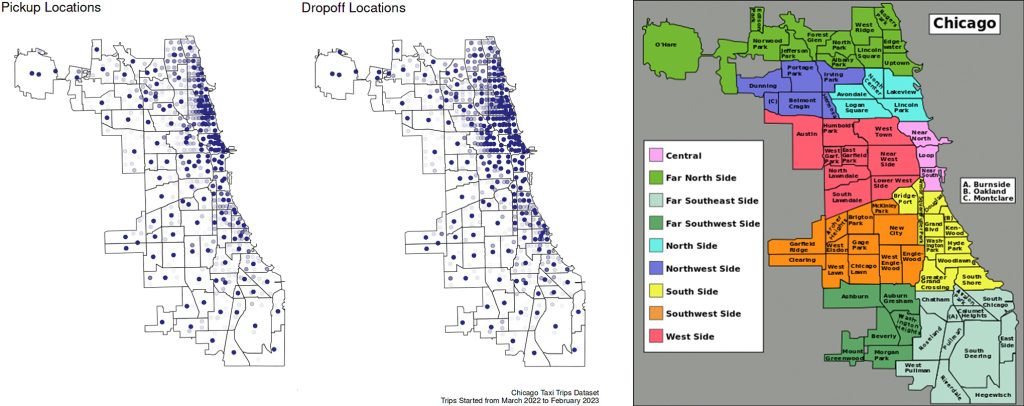
- Lakeview and Near North had the most varied pickup locations compared to other neighborhoods.
- While for dropoff locations, variations were mostly scattered in 4 neighborhoods: Lakeview, Near North, Lincoln Park, and West Town.
Relationship between two variables
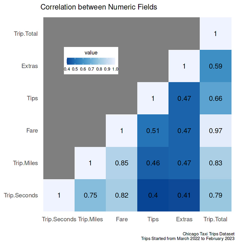
The interaction between the variables is in the figure above.
- The two variables with the highest correlation (0.97) were fare and total payment —meaning any other costs, e.g., tips, toll, and extras, insignificantly affected the whole amount.
- The distance (corrdistance.fare = 0.85, corrdistance.total = 0.83) slightly steered the travel cost compared to the duration of the trip (corrduration.fare = 0.82, corrduration.total = 0.79).
- The weakest correlation between numeric variables was between the trip duration and tips.
The correlation mentioned above will be discussed more in the next section.
Fare vs. total cost
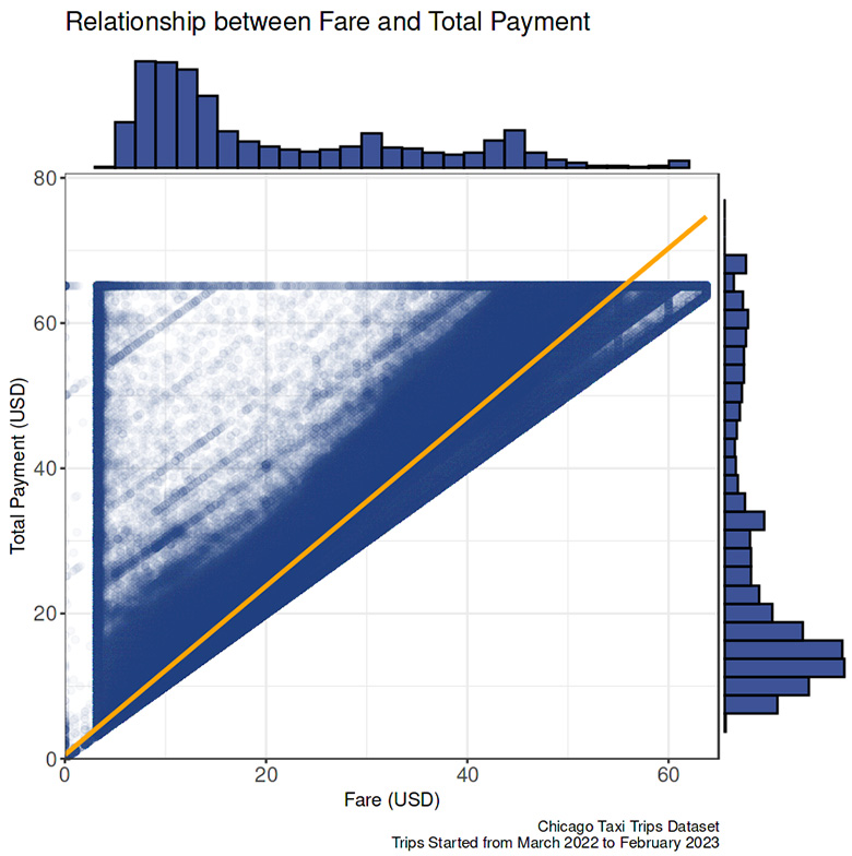
- Fare and total cost were significantly related. The observations condensed around the linear regression line.
- The blank space in the right below quadrant indicates that all total costs were equal or more pricey than the fare.
Fare vs. travel distance and duration
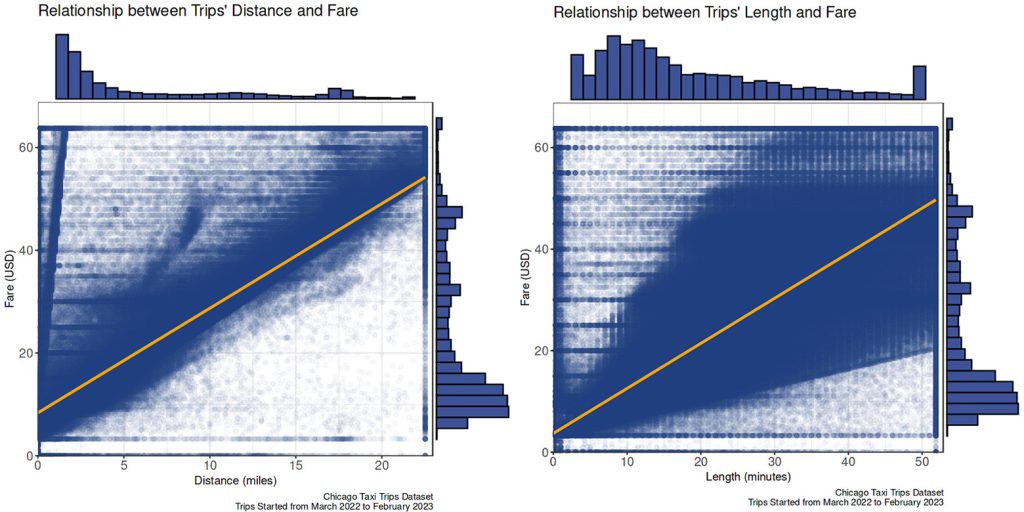
- The fare had a positive correlation with both travel distance and duration.
- The fare rose more constantly as the travel distance expanded compared to the travel duration extended. There was more variation in the fare if a passenger traveled longer in time.
The traffic probably causes it. If a passenger wants to reach the same destination, heavier traffic will slow down the trip than usual; hence same fare but longer travel time.
Travel time vs. distance
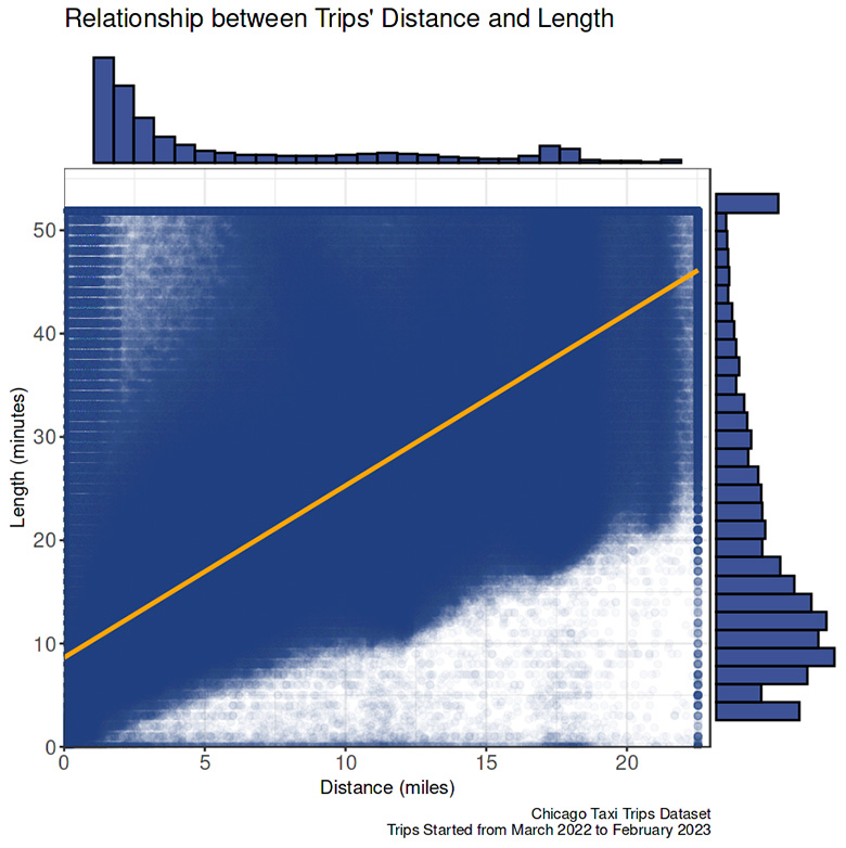
- The data were recorded in 15-minute aggregation; hence the travel time is clipped every 15 minutes in the graph.
- A moderately strong, positive, linear association exists between travel time and distance.
Travel time vs tips
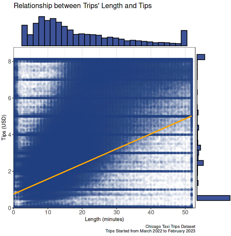
- Taxi riders are likely to pay the tips in the increment of 50 cents, regardless of the travel length, hence a weak association between these two variables.
Remarks and Recommendations
From the EDA, we can study the general mobility pattern of taxi trips in Chicago between March 2022 to February 2023. Three findings that entice me the most are listed below.
- During holidays such as Easter, Memorial Day, 4th of July, Labor Day, Thanksgiving, and Christmas, there were fewer taxi trips compared to the week before and after. >>
- The fare histogram shows multimodal peaks ranging from $8.5 to $9.5, $29.5 to $30.5, and $43.5 to $44.5. >>
- Lakeview and Near North neighborhoods had the most varied pickup locations, while variations in dropoff locations were mainly scattered across four neighborhoods: Lakeview, Near North, Lincoln Park, and West Town. >>
The information gathered from this EDA can be helpful for many applications. For instance, knowing that the most popular payment method is credit cards, taxi companies must ensure the card machine functions well in all taxis. Additionally, they can partner with credit card companies to offer more reward points to passengers who use their services. In Lakeview and Near North areas, where popular pickup spots are scattered, drivers may benefit from driving around to find passengers rather than waiting in one place. By implementing these recommendations, taxi companies may enhance passenger satisfaction, improve driver efficiency, and ultimately increase revenue.
References
- Chicago district map attribution: Peter Fitzgerald, CC BY-SA 3.0, via Wikimedia Commons
*As an Amazon Associate, I earn from qualifying purchases.